In my last post I demonstrated how to use Total Variation (TV) minimization to denoise a signal. Here I will show how the same concept can be used to reconstruct a signal from undersampled data in another domain. This works in the case where undersampling of a signal in one domain leads to noise-like artifact in a transform domain. Here I will use the case of sampling in the Fourier domain, where pseudo-random undersampling results in incoherent (noise-like) artifact in the transform domain.
Reconstruction from Fourier Samples
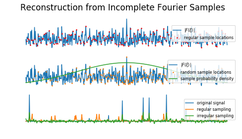
If a signal is fully-sampled, we can reconstruct from Fourier samples by a simple Fourier transform (or FFT). (For clarity: in this work I will refer to spatial domain signals (\(x\)) and spatial frequency representations (\(\xi\)), but the same applies to time domain signals.) In the case of undersampled data, a naïve reconstruction can be achieved using zero-filling for the unknown samples. The result is aliasing in the transform-domain signal. Aliasing takes many forms depending on the spacing of your samples: more gaps and bigger gaps between samples lead to more aliasing, regular spacing leads to coherent aliasing (aka wraparound, ghosting, etc.) but irregular spacing can make aliasing incoherent and noise-like.
A more informed reconstruction will recognize the missing samples are likely not simply zeros, which can reduce the appearance of aliasing. We want to find the signal that minimizes error from our actual samples in the transform domain, but we can incorporate additional information or assumptions about what our signal looks like to improve the solution. Some examples from medical imaging (my background is in magnetic resonance imaging) include using localized coil sensitivity maps (aka parallel imaging) and sparsity-promoting techniques (aka compressed sensing).
Total Variation Reconstruction
Looking back at the TV denoising examples from my last post, reconstruction is a fairly straightforward extension. At this point we can formalize the problem:
Where \(A\) represents Fourier undersampling, \(x\) is the image we're reconstructing, and \(b\) is the vector of undersampled Fourier measurements. Check out the figure below that compares a TV recon of the above 1D signal from undersampled (~3x) Fourier data for different values of the regularization parameter \(\lambda\).
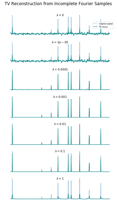
What this shows is that under certain circumstances -- the right undersampling pattern, the right regularization function and parameter, and an original signal with the right properties -- we can achieve perfect or near-perfect reconstruction. Maybe that's a lot of ifs, but the end result is nonetheless remarkable. For the specific case of TV reconstruction this also shows how if we choose \(\lambda\) too low we end up with residual (noise-like) aliasing, and too high we end up losing legitimate features (low contrast features drop out first). For now we can just consider \(\lambda\) to be determined empirically for a given application, but know that methods exist for tuning such parameters.
Image Reconstruction (TV in 2D)
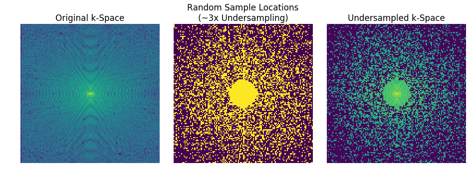
As you may expect, this can be extended to higher-dimensional data. For demonstration sake I will show how this works for images. First, let's look at the random undersampling of the Fourier data (aka k-space).
Now, my implementation is not lightning fast here, but it works. Here are the results after doing my own tweaking and settling on \(\lambda = 0.1\):
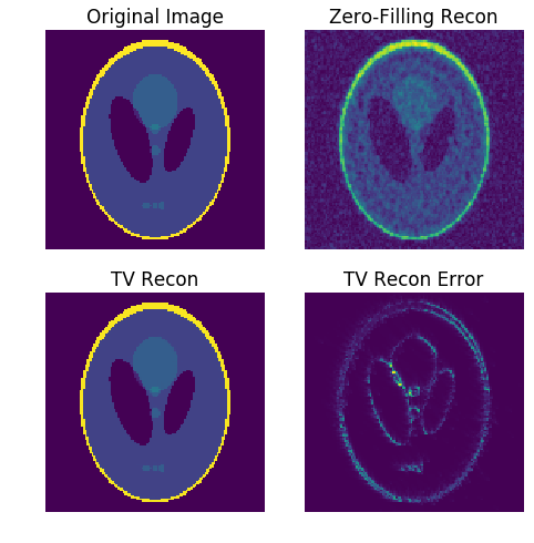
That's it! We have near-perfect image reconstruction from approximately 1/3 of the required Fourier coefficients. This is kind of like signal compression in reverse, and is referred to as Compressed Sensing. From here you can consider how other constraints besides TV may fit into this framework to allow even further undersampling.
At the time of posting it's a little messy, but if you're curious you can also play around with the Jupyter Notebook I used for this post.