Let's talk about nonlinear solvers, specifically the Alternating Directions Method of Multipliers (ADMM).
I've been reading through Steven Boyd's Convex Optimization book, as well as his (rather long) paper on ADMM. He has kindly posted a number of examples for this paper on his website to demonstrate how to write an ADMM solver. The examples are all in Matlab, but I typically work in Python so in the process of learning and playing with the examples I am also translating some to Python.
Total Variation Denoising
The example I'm going to demonstrate here is total variation denoising. One way I think about denoising is as a method of fitting a dense set of existing data (so no interpolation) while minimizing some added metric (regularization). The regularization term should be selected such that it penalizes noise while preserving the features in your signal. A regularization parameter (often \(\lambda\)) is used to tune the algorithm performance. There are a number of ways to do this, but one popular method is to add a penalty for the total variation of the signal. Total variation (TV) is the sum of absolute value of adjacent differences:
Formally, the whole denoising problem looks like this:
In plain(er) English: find a vector \(x\) that minimizes the sum-of-squares of the differences (aka least squares) between itself and the input \(b\) but also keep the TV of the new vector low. If \(\lambda\) is small prefer matching the input, if it is large prefer minimizing TV.
That's all well and good - but how is actually done in a practical sense? This is a huge field generally called optimization. Optimization problems can then of course be formalized and subcategorized. Generally speaking if an optimization problem is linear it can be solved, if it is "convex" it can very often be solved. Least-squares fitting is a linear problem. TV denoising is a convex problem.
ADMM
ADMM is a method for solving convex problems. The key to using ADMM is the separable terms in the minimization. This allows the whole problem to be solved by iterating over two subproblems, solving them alternatively with each iteration followed by a dual-variable update. Basically ADMM can solve (many) problems with the very general form:
OK that kind of looks like our TV denoising problem above, so we're on the right track. Now, we need two variables in ADMM but our problem only has one (\(x\)). This will seem silly, but to fix it we'll just make up the variable \(z\) and say \(Fx-z = 0\), where \(F\) is the matrix form of our TV operator.
Let's see if we can write our problem closer to the ADMM form now:
I'll be very explicit here about how these problems line up:
Right, now we can look at the ADMM algorithm that's going to solve our problem. It's an iterative solver, and here are the iteration update steps. Basically we will do these steps for some number of iterations, or until the solution seems like it's not changing much (probably close enough to solved):
Where \(L_{\rho} = f(x) + g(z) + y^T(Ax + Bz - c) + \frac{\rho}{2}\|Ax + Bz - c\|_2^2\) is the augmented Lagrangian of our problem. This formulation can help transform constrained optimization problems into unconstrained problems. For more information check out the ADMM paper linked above.
Since the objectives are separable, we can simplify the update steps a bit further (just shown for \(x\), but applies likewise to \(z\)):
But how is solving two optimization problems better than one? This method works because each of the subproblems is much easier to solve than our original problem. Notice with each individual update we're only minimizing with respect to one variable - since our objective function is separable, this greatly simplifies the problem.
Show the Code
As mentioned, this is mostly a Matlab-to-Python translation of Steven Boyd's example, but I have also played around with a few different tweaks. Anyway let's get started with some familiar imports.
import numpy as np
import scipy.sparse
import matplotlib.pyplot as plt
Next let's do a straight port of the Matlab code, going through it piece-by-piece. Let's start with the function definition, docstring (basically plagiarized from the example), and some constants used for stopping criteria.
def total_variation(b, lam, rho, alpha):
    """ Solve total variation minimization via ADMM

    Solves the following problem via ADMM:

       min  (1/2)||x - b||_2^2 + lambda * sum_i |x_{i+1} - x_i|

    where b in R^n.

    The solution is returned in the vector x.

    history is a structure that contains the objective value, the primal and
    dual residual norms, and the tolerances for the primal and dual residual
    norms at each iteration.

    rho is the augmented Lagrangian parameter.

    alpha is the over-relaxation parameter (typical values for alpha are
    between 1.0 and 1.8).

    More information can be found in the paper linked at:
    http://www.stanford.edu/~boyd/papers/distr_opt_stat_learning_admm.html

    *Code adapted from Steven Boyd*
    https://web.stanford.edu/~boyd/papers/admm/total_variation/total_variation.html"""

    MAX_ITER = 1000
    ABSTOL = 1e-4
    RELTOL = 1e-2
The following chunk of code is some variable initialization, and we pre-calculate the (sparse) difference matrix \(D\) used for calculating TV, as well as the product with its own transpose (\(DtD\)) which will be used later.
    ...

    n = len(b)

    if np.ndim(b) == 1:
        b = b[:, None]

    e = np.ones(n)

    # difference matrix
    D = scipy.sparse.spdiags(np.vstack((e, -e)), (0, 1), n, n)
    DtD = D.T @ D

    # sparse identity matrix
    I = scipy.sparse.eye(n, format='csc')

    x = np.zeros((n, 1))
    z = x.copy()
    u = x.copy()

    history = {'objval' : [],
               'r_norm': [],
               's_norm': [],
               'eps_prim': [],
               'eps_dual': []}
Here's the ADMM algorithm itself showing the \(x\), \(z\), and \(y\) (\(u\)) updates. Here is where Chapter 4 in the ADMM paper referenced above is very helpful in describing methods for solving the sub-problems based on the form of the objective terms. The \(x\) update is for the \(f(x)\) term and we're using a "direct method" to solve it since the objective is quadratic (see 4.2). The \(z\) update uses soft thresholding (see 4.4.3) since the \(g(z)\) objective is to minimize the L1 norm. This implementation also makes use of the scaled dual variable \(u=y/\rho\) (3.1.1) and (over-)relaxation with the parameter alpha, which can improve convergence (3.4.3).
    ...

    for k in range(MAX_ITER):

        # x-update (minimization) for (1/2)||x - b||_2^2
        # uses a direct method for the quadratic objective term
        x = spsolve((I + rho * DtD), (b + rho * D.T.dot(z - u)))

        # z-update (minimization) with relaxation for lam * ||z||_1
        # uses soft thresholding for the L1 term
        # see ADMM paper 3.4.3
        z_ = z
        Ax_hat = alpha * D @ x + (1 - alpha) * z_
        z = shrinkage(Ax_hat + u, lam / rho)

        # y-update (dual update)
        # u is the scaled dual variable y/rho (ADMM paper 3.1.1)
        u = u + Ax_hat - z
With the updates out of the way, we will keep track of some calculated values in the history dictionary to evaluate performance and convergence. Finally we will check for convergence based on both absolute and relative tolerances of the primal and dual residuals.
    ...
        ...

        # keep track of progress
        objval = TV_denoising_objective(b, lam, x, z)

        r_norm = np.linalg.norm(D @ x - z)
        s_norm = np.linalg.norm(-rho * D.T @ (z - z_))

        eps_prim = np.sqrt(n) * ABSTOL + RELTOL * max(np.linalg.norm(D @ x),
                                                      np.linalg.norm(-z))
        eps_dual = np.sqrt(n) * ABSTOL + RELTOL * np.linalg.norm(rho * D.T @ u)

        history['objval'].append(objval)
        history['r_norm'].append(r_norm)
        history['s_norm'].append(s_norm)
        history['eps_prim'].append(eps_prim)
        history['eps_dual'].append(eps_dual)

        if r_norm < eps_prim and s_norm < eps_dual:
            break

    return history, x
Lastly, there are two small functions used above that we will still need to define: the objective value is a straightforward code implementation of our stated problem, and the shrinkage function is used for soft-thresholding (moves all values of its input toward 0).
def TV_denoising_objective(b, lam, x, z):
    """TV denoising objective calculation"""
    return 0.5 * np.linalg.norm(x - b)**2 + lam * np.linalg.norm(z)

def shrinkage(a, kappa):
    """Soft-thresholding of `a` with threshold `kappa`"""
    return np.clip(a-kappa, a_min=0, a_max=None) - np.clip(-a-kappa, a_min=0, a_max=None)
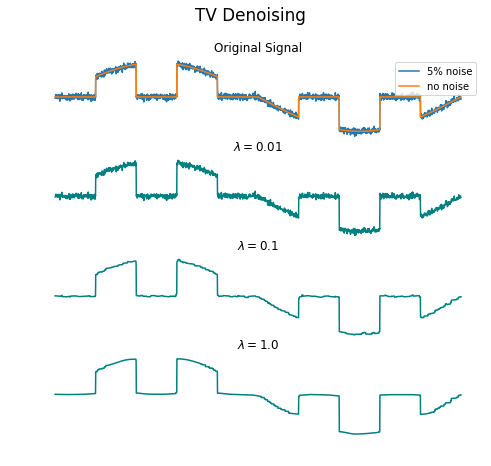
Great, now we're ready to run it and see how it works. We'll try it with three different values for \(\lambda\).
%time hist, x = total_variation(b_, 0.01, 1.0, 1.0)
CPU times: user 424 ms, sys: 24 ms, total: 448 ms
Wall time: 449 ms

%time hist, x = total_variation(b_, 0.1, 1.0, 1.0)
CPU times: user 433 ms, sys: 11.3 ms, total: 445 ms
Wall time: 445 ms

%time hist, x = total_variation(b_, 1.0, 1.0, 1.0)
CPU times: user 1.06 s, sys: 16.1 ms, total: 1.07 s
Wall time: 1.08 s
A Matrix-Free Implementation
It's nice when you can form a matrix operator and take advantage of existing clever linear algebra algorithms to efficiently compute things, but this is not always practical. Especially when dealing with (vectorized) images, for example, where even sparse matrices can be difficult to form or store efficiently. Additionally, many linear transformations - such as spatially variant blurring - don't have convenient (i.e. structured and/or sparse) matrix forms. This is where matrix-free methods come into play. Often we don't actually need a matrix if we can calculate matrix-vector products.
SciPy has some helpful features here in scipy.sparse.linalg. Note specifically the LinearOperator class, that lets you define a linear operator by specifying functions for \(Av\) (matvec) and \(A^Hv\) (rmatvec). Using a LinearOperator instead of a matrix means we can no longer use solve or inv, but we get our choice of built in solvers. Below I just use cg (conjugate gradient) since the matrix we're inverting (\(I + \rho D^HD\)) is symmetric and positive semidefinite.
from scipy.sparse.linalg import LinearOperator, cg

def matrix_free_tv(b, lam, rho, alpha):
    """ Solve total variation minimization via ADMM *without forming the difference matrices*

    Solves the following problem via ADMM:

       min  (1/2)||x - b||_2^2 + lambda * sum_i |x_{i+1} - x_i|

    where b in R^n.

    The solution is returned in the vector x.

    history is a structure that contains the objective value, the primal and
    dual residual norms, and the tolerances for the primal and dual residual
    norms at each iteration.

    rho is the augmented Lagrangian parameter.

    alpha is the over-relaxation parameter (typical values for alpha are
    between 1.0 and 1.8).

    More information can be found in the paper linked at:
    http://www.stanford.edu/~boyd/papers/distr_opt_stat_learning_admm.html

    *Code adapted from Steven Boyd*
    https://web.stanford.edu/~boyd/papers/admm/total_variation/total_variation.html"""
    MAX_ITER = 1000
    ABSTOL = 1e-4
    RELTOL = 1e-2

    n = len(b)

    def D(v):
        return v - np.roll(v, -1)

    def Dt(v):
        return v - np.roll(v, 1)

    def mv(v):
        # return v + rho * (2*v - np.roll(v, -1) - np.roll(v, 1))
        # return v + rho * DtD @ v
        return v + rho * Dt(D(v))

    F = LinearOperator((n,n), matvec=mv, rmatvec=mv)

    x = np.zeros((n,))
    z = x.copy()
    u = x.copy()

    history = {'objval' : [],
               'r_norm': [],
               's_norm': [],
               'eps_prim': [],
               'eps_dual': []}

    for k in range(MAX_ITER):

        # x-update (minimization)
        # iterative version
        x, _ = cg(F, b + rho * Dt(z - u), maxiter=100, x0 = x)

        # z-update (minimization) with relaxation
        # uses soft thresholding - the proximity operator of the l-1 norm
        z_ = z
        Ax_hat = alpha * D(x) + (1 - alpha) * z_
        z = shrinkage(Ax_hat + u, lam / rho)

        # y-update (dual update)
        u = u + Ax_hat - z

        # keep track of progress
        objval = objective(b, lam, x, z)

        r_norm = np.linalg.norm(D(x) - z)
        s_norm = np.linalg.norm(-rho * z - z_ - np.roll(z - z_, 1))

        eps_prim = np.sqrt(n) * ABSTOL + RELTOL * max(np.linalg.norm(D(x)),
                                                      np.linalg.norm(-z))
        eps_dual = np.sqrt(n) * ABSTOL + RELTOL * np.linalg.norm(rho * Dt(u))

        history['objval'].append(objval)
        history['r_norm'].append(r_norm)
        history['s_norm'].append(s_norm)
        history['eps_prim'].append(eps_prim)
        history['eps_dual'].append(eps_dual)

        if r_norm < eps_prim and s_norm < eps_dual:
            break

    return history, x
Now I'll run this again with the same three \(\lambda\) values from the original version:
%time hist, x = matrix_free_tv(b_, 0.01, 1.0, 1.0)
CPU times: user 343 ms, sys: 273 µs, total: 344 ms
Wall time: 344 ms

%time hist, x = matrix_free_tv(b_, 0.1, 1.0, 1.0)
CPU times: user 380 ms, sys: 2.33 ms, total: 382 ms
Wall time: 382 ms

%time hist, x = matrix_free_tv(b_, 1.0, 1.0, 1.0)
CPU times: user 512 ms, sys: 3.7 ms, total: 515 ms
Wall time: 513 ms
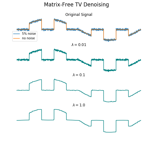
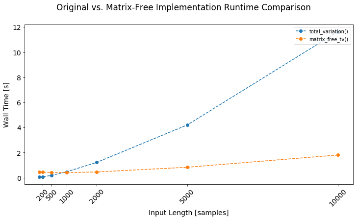
The results are similar but not quite identical, so I'm guessing my LinearOperator is incorrect by a bit somewhere. However, the matrix-free version actually seems slightly better at preserving the flatness in the valleys. This version is also significantly faster with increasing input length, though it's notable the matrix implementation is faster for small inputs (runtime also changes with \(\lambda\)). Of course neither implementation is necessarily optimized - this is more of a casual observation about my initial naïve implementations. The ADMM paper gives some additional recommendations for speeding things up when using direct (as in the first implementation above) or iterative (as with my matrix-free implementation) techniques.
Why TV Anyway?
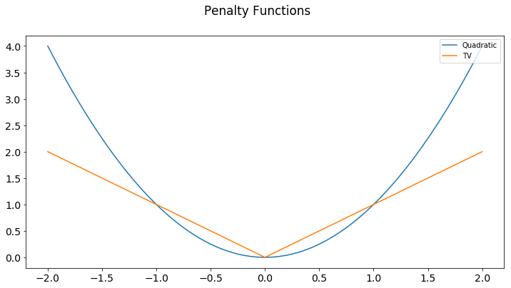
Why use total variation anyway? The good thing about total variation is its ability to preserve the sharp edges in our signal. Check out what quadratic smoothing looks like in comparison:
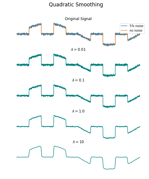
This all comes down to the shape of the penalty function. With a quadratic penalty, small changes are tolerated while large deviations are severely penalized. With a TV (L1) penalty, deviations are all penalized proportionally to their size. Hopefully this lends some intuition to the methods.
Conclusion
So that's TV denoising implemented via ADMM. I also implemented the quadratic smoothing function with ADMM, and you can check that along with all the other code used to create this post in the associated Jupyter Notebook.